Calculate Fourier parameters from shape data

In this tutorial we take a look at how to construct Harmonica’s Fourier parameterisation of a transmission string from shape data. This is useful for forward modelling transit light curves of various objects with known shapes. You only need to determine some high-order Fourier representation of the shape, and then you may easily simulate high-precision light curves.

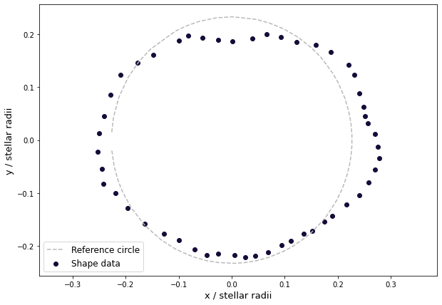
Let us start by loading some shape data. Here is some data made earlier, based on the transit of Phobos as viewed from the Perseverance rover on Mars.

import numpy as np
import matplotlib.cm as cm
import matplotlib.pyplot as plt


r_data = np.array([ 0.25299594, 0.25049962, 0.2555872 , 0.24131962, 0.23499399, 0.2281387 , 0.21770261, 0.21355986, 0.21756298, 0.22216417, 0.215748  , 0.21737008, 0.22181932, 0.22220379, 0.22215942, 0.2191899 , 0.22060524, 0.22316191, 0.22795516, 0.23203883, 0.23715028, 0.24817015, 0.26129245, 0.2701211 , 0.27631858, 0.279554  , 0.27550068, 0.26970037, 0.25844681, 0.2551263 , 0.2564253 , 0.25649795, 0.2619272 , 0.26137834, 0.24959362, 0.23925815, 0.2218478 , 0.21541933, 0.21006674, 0.1952882 , 0.18672611, 0.19014673, 0.20044651, 0.2134876 , 0.21243847, 0.21826262, 0.23046709, 0.24290151, 0.24455098, 0.24425059, 0.25006916])
theta_data = np.array([-3.05626382, -2.92458806, -2.81512117, -2.71398938, -2.56361121, -2.37500762, -2.19475882, -2.05340439, -1.89915229, -1.78311113, -1.68792003, -1.54576688, -1.45830389, -1.36707739, -1.26004262, -1.12498761, -1.03931859, -0.91754355, -0.8460734 , -0.72241586, -0.64825102, -0.51378753, -0.40700302, -0.30187693, -0.20512046, -0.1247507 , -0.0469304 , 0.04035871, 0.12437005, 0.17993957, 0.24397848, 0.35182409, 0.48800481, 0.57248726, 0.72834884, 0.84510295, 0.98657143, 1.12488908, 1.2518673 , 1.36829014, 1.56557413, 1.70233616, 1.84736078, 1.96211635, 2.0600249 , 2.31436316, 2.4535093 , 2.60749337, 2.78292412, 2.95552791, 3.08844006])

plt.figure(figsize=(10, 7))
plt.gca().set_aspect("equal", "datalim")
plt.scatter(r_data * np.cos(theta_data), r_data * np.sin(theta_data),
            color=cm.inferno(0.1), label="Shape data")
plt.plot(0.2267 * np.cos(theta_data), 0.2324 * np.sin(theta_data),
         color="#b9b9b9", ls="--", label="Reference circle")
plt.xlabel("x / stellar radii", fontsize=13)
plt.ylabel("y / stellar radii", fontsize=13)
plt.legend(loc="lower left", fontsize=12)
plt.show()

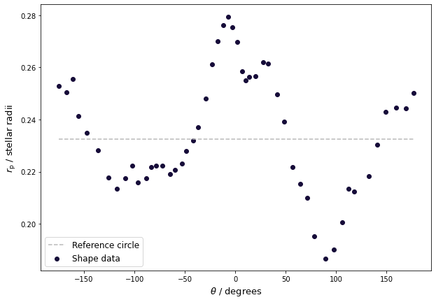
In polar coordinates:

plt.figure(figsize=(10, 7))
plt.scatter(theta_data * 180. / np.pi, r_data,
            color=cm.inferno(0.1), label="Shape data")
plt.plot(theta_data * 180. / np.pi, 0.2324 * np.ones(theta_data.shape[0]),
         color="#b9b9b9", ls="--", label="Reference circle")
plt.xlabel("$\\theta$ / degrees", fontsize=13)
plt.ylabel("$r_{\\rm{p}}$ / stellar radii", fontsize=13)
plt.legend(loc="lower left", fontsize=12)
plt.show()

The Fourier parameters of Harmonica’s transmission strings can be calculated from these data. This involves solving:

\[a_0 = \frac{1}{2 \pi} \int_{-\pi}^{\pi} r(\theta) \,d \theta,\]

\[a_n = \frac{1}{\pi} \int_{-\pi}^{\pi} r(\theta) \cos{(n \theta)} \,d \theta,\]

\[b_n = \frac{1}{\pi} \int_{-\pi}^{\pi} r(\theta) \sin{(n \theta)} \,d \theta,\]

where each integrand is a generated interpolation function based on the data. You can compute these coefficients up to a high order, although be careful of going too far as numerical ringing starts to appear. Here let us compute up to \(n = 10\).

from scipy import interpolate, integrate


transmission_string_params = []
for n in range(11):

    if n == 0:
        # a_0 term.
        integrand_cos0_func = interpolate.interp1d(
            theta_data, r_data,
            kind="cubic", bounds_error=False, fill_value="extrapolate")
        cn = integrate.quad(
            integrand_cos0_func, -np.pi, np.pi,
            epsabs=1.e-7, epsrel=1.e-7, limit=500)[0] / (2. * np.pi)
        transmission_string_params.append(cn)
    else:
        # a_n terms.
        integrand_cosn_func = interpolate.interp1d(
            theta_data, r_data * np.cos(n * theta_data),
            kind="cubic", bounds_error=False, fill_value="extrapolate")
        cn = integrate.quad(
            integrand_cosn_func, -np.pi, np.pi,
            epsabs=1.e-7, epsrel=1.e-7, limit=500)[0] / (1. * np.pi)
        transmission_string_params.append(cn)

        # b_n terms.
        integrand_sinn_func = interpolate.interp1d(
            theta_data, r_data * np.sin(n * theta_data),
            kind="cubic", bounds_error=False, fill_value="extrapolate")
        sn = integrate.quad(
            integrand_sinn_func, -np.pi, np.pi,
            epsabs=1.e-7, epsrel=1.e-7, limit=500)[0] / (1. * np.pi)
        transmission_string_params.append(sn)

transmission_string_params = np.array(transmission_string_params)

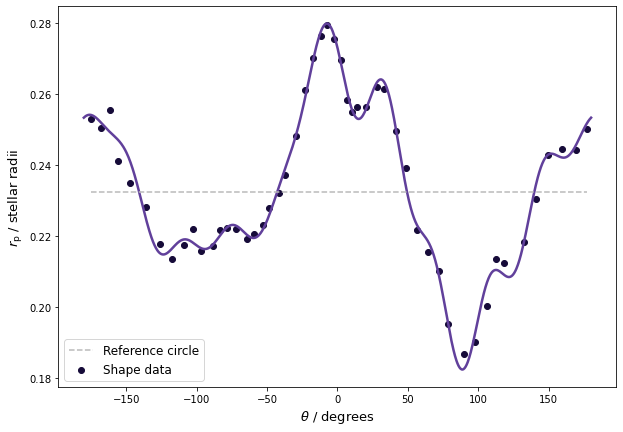
Now plot the resulting transmission string and check you have a good approximation of your input shape:

from harmonica import HarmonicaTransit


ht = HarmonicaTransit()
ht.set_planet_transmission_string(transmission_string_params)
theta = np.linspace(-np.pi, np.pi, 1000)

plt.figure(figsize=(10, 7))
plt.plot(theta * 180. / np.pi, ht.get_planet_transmission_string(theta),
         c=cm.Purples(0.8), lw=2.5)
plt.scatter(theta_data * 180. / np.pi, r_data,
            color=cm.inferno(0.1), label="Shape data")
plt.plot(theta_data * 180. / np.pi, 0.2324 * np.ones(theta_data.shape[0]),
         color="#b9b9b9", ls="--", label="Reference circle")
plt.xlabel("$\\theta$ / degrees", fontsize=13)
plt.ylabel("$r_{\\rm{p}}$ / stellar radii", fontsize=13)
plt.legend(loc="lower left", fontsize=12)
plt.show()

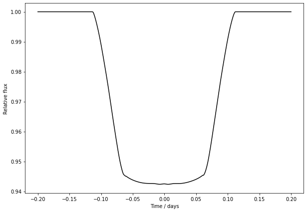
These parameters can now be used to generate transit light curves of your object. The only thing left to do is specify the orbit and stellar limb darkening.

times = np.linspace(-0.2, 0.2, 500)
ht = HarmonicaTransit(times)
ht.set_orbit(t0=0., period=4., a=7., inc=88. * np.pi / 180.)
ht.set_stellar_limb_darkening(u=np.array([0.074, 0.193]), limb_dark_law="quadratic")
ht.set_planet_transmission_string(transmission_string_params)
light_curve = ht.get_transit_light_curve()

plt.figure(figsize=(10, 7))
plt.plot(times, light_curve, c="#000000")
plt.xlabel('Time / days')
plt.ylabel('Relative flux')
plt.show()